

In the past, I’ve experimented with various forms of machine learning models in order to develop a successful cryptocurrency trading strategy. These various strategies would utilize classification models, time-series models, and sentiment analysis. The results of these strategies would range from mediocre to “good but requires more testing”. I’ve never settled on a specific strategy and hope to one day move on from the testing phase to “actually implementing it with real money” phase.
In all of these different strategies, I have yet to change the frequency of the historical data tested. The frequency of data I have always used and backtested with was the daily historical price data. That frequency for price data is not bad at all but it is limited, especially with the around the clock trading availability of the cryptocurrency market.
So in order to continue my testing, I’ll need to know what it is like to day trade crypto with machine learning. Specifically, I’ll be using a time series machine learning model that I have found to be easy to use and implement — Facebook Prophet. Feel free to code along with me or just continue reading to see the final outcome.
The Necessary Libraries and Data
To begin, I’ll need to import some libraries:
from eod import EodHistoricalData
import pandas as pd
from datetime import datetime, timedelta
import calendar
from tqdm import tqdm
import numpy as np
import random
import plotly.express as px
from prophet import Prophet
If you’re familiar with data science, then you may recognize many of these libraries.
Crypto Intraday Price Data
Next, I’ll have to grab the intraday price data for a selected cryptocurrency. To do so, I utilized a financial API service called EOD HD, which allows me to retrieve the historical price data of select cryptocurrencies at various time intervals. Disclosure: I earn a small commission from any purchases made through the link above.
# Importing and assigning the api key
with open("../../eodHistoricalData-API.txt", "r") as f:
    api_key = f.read()

# EOD Historical Data client
client = EodHistoricalData(api_key)
With my provided API key, I can now retrieve the hourly price data from assorted cryptocurrencies. For this project, I chose to focus on the most famous of crypto of them all — Bitcoin.
Function for Intraday Crypto Price Data
For this function, I’ll be grabbing the hourly price data. However, there are other options for shorter time intervals. At times during the API call, I found there to be a slight time delay. The API does have a separate package that provides live data but for the purpose of this project it was not necessary.
Next, I retrieved the hourly data from a specific timestamp dictated by the provided parameters within the function. After grabbing the data and performing some basic formatting and handling of missing data, I moved on to applying a moving average to the dataset. This is done in order to smooth out any outliers that may appear within the data. Lastly, the DataFrame is then renamed to be compatible with Facebook Prophet.
Training and Predicting with Facebook Prophet
I’ve written other articles detailing the process of training and predicting with Facebook Prophet on daily data. If you choose to learn more about that specific process then click here. However, in this project, I had to make adjustments to the function in order to compensate for the hourly data:
There are only two adjustments that needed to be made in order to handle intraday or hourly data. One was switching all the seasonality options to False. The other one was designating the frequency parameter to hourly with “H” within the .make_future_dataframe() function. Finally, this function returns the dates and predictions based on the provided DF.
Predictions Over Time
The next step would be to make predictions over a set period of time. To do so, I created a function that implements the train and predict function in a loop to simulate these predictions over time.
This function returns all the predictions made over the set period of time. For example, if the forecast_hours parameter is set to 5, then each date will have the predicted price of the fifth hour in the future. The function only trains on a moving window of the most recent hourly data in the ‘for’ loop, then makes a price forecast of 5 hours. I then shift these predictions back so that they will align with the “current” values. This is done to simulate what predictions could look like every hour if it were ran in realtime.
Now with the predictions and their respective “current” values set in a dataframe, I can move on to establishing the trading positions…
Trading Positions
The function above establishes the basic trading strategy used during the backtest. Here, if the “open” price of Bitcoin is less than the predicted lower bound price, then the returned position is a “Buy” or “1” and vice-versa. If it is neither then it basically means the position is a “0” or do nothing. These positions will make up the Prophet positions for the backtest.
Baseline Positions
The next thing I need to do is establish the baseline positions for the backtest. These positions will be used to compare to the Prophet positions in order to see if there are any significant improvements with using Prophet over them. These baseline trading strategy positions will be Buying and Holding and Random positions:
# Adding sentiment positions to the forecast DF
positions = pred_df

# Getting forecast prophet positions
positions['fbp_positions'] = positions.apply(
    lambda x: fbpPositions(x, short=True),
    axis=1
)

# Buy and hold position
positions['buy_hold'] = 1

# Random positions
positions['random_positions'] = random.choices(
    [1,0,-1], k=len(positions)
)
Performing the Backtest
With the positions ready to go, the final thing to do is to get the hour-by-hour returns. This is done by using the logarithmic returns on the ‘open’ prices:
# Getting returns each hour
log_returns = prices[['ds', 'open']].set_index(
    'ds'
).loc[positions.index].apply(np.log).diff()
With the log returns set, all I have left to do is multiply the returns with the positions DataFrame from before:
# The positions to backtest (shifted ahead by 1 to prevent lookahead bias)
bt_positions = positions[[
    'buy_hold',
    'random_positions',
    'fbp_positions'
]].shift(1)

# The returns during the backtest
returns = bt_positions.multiply(
    log_returns['open'],
    axis=0
)

# Inversing the log returns to get daily portfolio balance
performance = returns.cumsum().apply(
    np.exp
).dropna().fillna(
    method='ffill'
)
The backtest is complete! The results of which are stored within the performance variable. However, in order to quickly run different parameters for the backtest, I’ll need to consolidate all of these functions into one which will also include a visualization of the backtest after it has been completed.
Final Backtest Function
The above function consolidates the previous functions and will retrieve data, run predictions, establish trading positions, run the backtest, then return the final numbers and visualization.
Backtesting Visualization
With the following parameters:
backtestPerformanceVis(
    ticker="BTC",
    n_hours=300,
    training_hours=200,
    mov_avg=5,
    forecast_hours=5
)
I was able to achieve the following results:
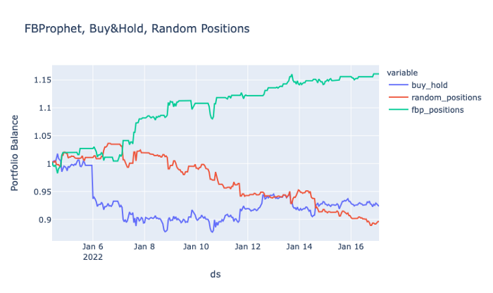
Closing Thoughts
Based on these results, it looks like Prophet would’ve performed very well in the previous 300 hours. It resulted in a return of 16% in about 300 hours! However, this could be a fluke and may require further testing of different parameters to really assess the robustness of this strategy.
With the final function I created, I can attempt other parameters such as increasing the backtesting length, increasing the training amount, or alter the moving average. Or even with the strategy itself, I can decide different positions based on the predictions. There are many different scenarios that should be tested before this strategy could be used in a real-time trade. But, as of now, the results are much more promising than I would have expected.