
A first algorithmic strategy with Grademark
JavaScript can be used for many things that you might not have thought of, including quantitative trading – in this blog post I show how to backtest a quantitative and systematic trading strategy with JavaScript.
As you might imagine this can be quite a complex topic, but in this post I’m only going to cover the basics and we are only going to look at a very simple and naive trading strategy.
In this post you will learn:
- How to define rules in JavaScript to implement a trading strategy;
- How backtesting works; and
- How to use Grademark to simulate trading and analyze the performance of a strategy.
If you want to jump ahead for a sneak peek at the backtest we are creating in this blog post please look here. That notebook was created with Data-Forge Notebook and that’s how I created the charts in this blog post. You can find a version of the example code for Node.js on GitHub.
Don’t worry if you don’t know much about JavaScript… the code snippets included in this post are pretty simple and for the moment it’s enough if you can just read them and generally get the gist of what’s being done.
For more content like this, follow Ashley Davis on Twitter.
Also I’m planning a book on this subject that might interest you: Backtesting and algorithmic trading with JavaScript.
Video content
This blog post is basically a written version of some videos that I’ve already created. You can continue to read about it here or you can watch the videos instead.
The first video is a primer on trading and covers some of the basics and theory of backtesting using JavaScript.
The second video is a demonstration using Data-Forge Notebook that shows how to test a simple strategy in JavaScript.
What is Grademark?
Grademark is my open-source toolkit for backtesting and quantitative trading. If you like the sound of it please star the repo.
Why quantitative trading?
When I say quantitative trading, what I mean is systematic trading by the numbers.
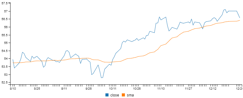
When developing our trading strategy we will start by defining indicators that we’ll use as trading signals. The only indicator I’m using as an example in this post is a simple moving average derived from daily close price. This is illustrated in the following chart:

Our trading strategy consists of a system of rules we use to decide, based on our indicators, when we should open and close trades. We also define rules to help us manage the risk. We thus create a systematic strategy, one that can be simulated.
owing chart:
Our trading style is a very personal choice and must be aligned with our goals and financial strategy. I prefer systematic quantitative trading strategies for the following reasons:
- It takes the emotion out of trading;
- It can be simulated;
- Performance can be tested; and
- Trading can be automated.
It’s the last reason that’s most appealing. It’s the dream of any systematic trader to be able to go fully algorithmic, putting our strategy on automatic then retiring to a beach with a cocktail in hand.
Why simulate?
There are many reasons to simulate trading, not just to test the performance of your strategy.
We might want to simulate trading to
- Practice trading and gain confidence/experience in the market, but in a risk-free environment;
- Prepare for trading when you don’t yet have the capital for real trading;
- Evaluate alternative strategies;
- Figure out how to manage risks and survive worst-case scenarios;
- Understand a particular market or financial instrument; and importantly
- Prepare yourself for the psychological aspects of trading (handling losses)
As you can see there are many reasons why simulation is useful. I’m sure you can think of more.
Managing risk
An important aspect of trading (and hence of trading simulation) is learning how to manage risk.
When I talk about risk I’m talking about the risk of losing money. Losing is a part of the game and it’s ok provided your eventual wins outweigh your losses. That’s how we can make a profit.
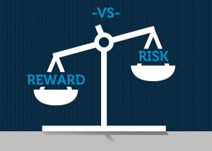
Simulation can help us here in two ways. It can help us prepare for the psychological impact of losing. It also shows whether the wins from our strategy can overpower the losses and how well our strategy copes with occasional disastrous market corrections.
Types of simulation
There are actually two main ways to simulate trading. Paper trading and backtesting. Paper trading is also known as forward testing.
Paper trading happens in real time, is very realistic and can feel much like real trading. I highly recommend that beginners start with paper trading. It’s a great way to start building your experience in the market.
Unfortunately, paper trading is very slow. It happens in real time, which means that if you are simulating a medium- to long-term trading strategy it would take months if not years to yield results.
Paper trading is easy and realistic. It’s a good starting point, but is also very slow.
This is where backtesting comes to our rescue. It’s called backtesting because it tests a trading strategy on historical data. It’s going backward in time to find out what would have happened if you had executed your strategy in the real market in the past.
It’s more complicated than paper trading and you are going to need some programming skills to do it. Backtesting wins though because it delivers results very quickly. Through backtesting, we can simulate our strategy and analyze the results just as quickly as our computer program can process all the data. Having optimized code and a fast computer will help here, but anyway you look at it – backtesting delivers results very quickly compared to paper trading.
A short and simple backtest will take minutes. More complex strategies, bigger markets and more data increase the amount of time required. But we are still talking about having a result in hours or days, rather than in weeks, months or even years.
Backtesting is more complicated, but is vastly quicker than paper trading.
Loading and preparing input data
Before backtesting our trading strategy we need to load and prepare historical price data.
We can use Data-Forge to load the data into a dataframe:
let inputSeries = dataForge.readFileSync("data/STW.csv")
.parseCSV()
.parseDates("date", "D/MM/YYYY")
.parseFloats(["open", "high", "low", "close", "volume"])
// Index so we can soon merge on date.
.setIndex("date")
// Rename "date" to "time" for Grademark.
.renameSeries({ date: "time" });
We now need to compute an indicator to use as a trading signal. Our mean reversion strategy calls for a moving average. So let’s compute that from our input data:
const movingAverage = inputSeries
.deflate(bar => bar.close) // Extract closing price series.
.sma(30);                  // 30 day moving average.
Grademark expects that we’ll have all our input data and indicators combined. So we must now merge our moving average indicator into the input data:
// Integrate moving average indexed on date.
inputSeries = inputSeries.withSeries("sma", movingAverage)
    .skip(30); // Skip blank sma entries.
Our input data is in the inputSeries variable and ready to be used in backtesting.
It’s always good to visualize our data after doing such computations to ensure that it looks like what we expect and that we don’t have any bugs in our code. I originally put this code together in Data-Forge Notebook which allowed me to very conveniently visualize the input data:
Entering a position
Now that we have some data we can put together the code for our strategy.
The first bit of code is a rule that determines when we should open a trade and take a position.
Our example mean reversion trading strategy is simple, so our code to open a position is also simple:
if (args.bar.close < args.bar.average) {
      enterPosition();
}
This code opens a trade by calling the enterPosition function when the closing price is less than the average price. This function is provided by Grademark. The args variable is provided for us by Grademark and gathers together pertinent details of the trading environment such as the latest bar of price action.
Exiting a position
Closing a trade – exiting our position – is the reverse of entering it:
if (args.bar.close > args.bar.average) {
      exitPosition();
}
Here we are saying that when the closing price is above the average price, then we exit the position immediately.
I know what you are thinking: can something so simple and naive actually produce a profit?
Stay tuned, very soon we’ll find out.
Stop loss rule
When I’m trading I also like to use a stop loss rule to help limit losses and manage risk. A stop loss rule is a different kind of exit, one that kicks in to stop us from losing more than a certain amount of money.
In the following stop loss rule I’m setting a maximum loss of 2% per position before exiting:
const stopDistancePct = 2;
const stopPrice =
	args.entryPrice - (args.entryPrice * (stopDistancePct/100));
if (args.bar.close <= stopPrice) {
	exitPosition();
}
Note that we are calling the same exitPosition function as we did in our exit rule. A stop loss is just another way of exiting a position.
Using a stop loss is considered by some traders to erode profit potential for a strategy. So why do I like to use this rule? I like to use this rule in real trading as I feel it protects me against the heaviest losses. It buys me some peace of mind. In real trading I have a stop loss rule automatically applied by my broker and this means I can go on holiday and know that my investments are protected.
In this example, I’ve included the stop loss right from the start, but normally you might consider this as an incremental addition to the strategy, testing before and after adding it – normally you’d probably like to know how much of a difference the stop loss makes to understand if it is worthwhile.
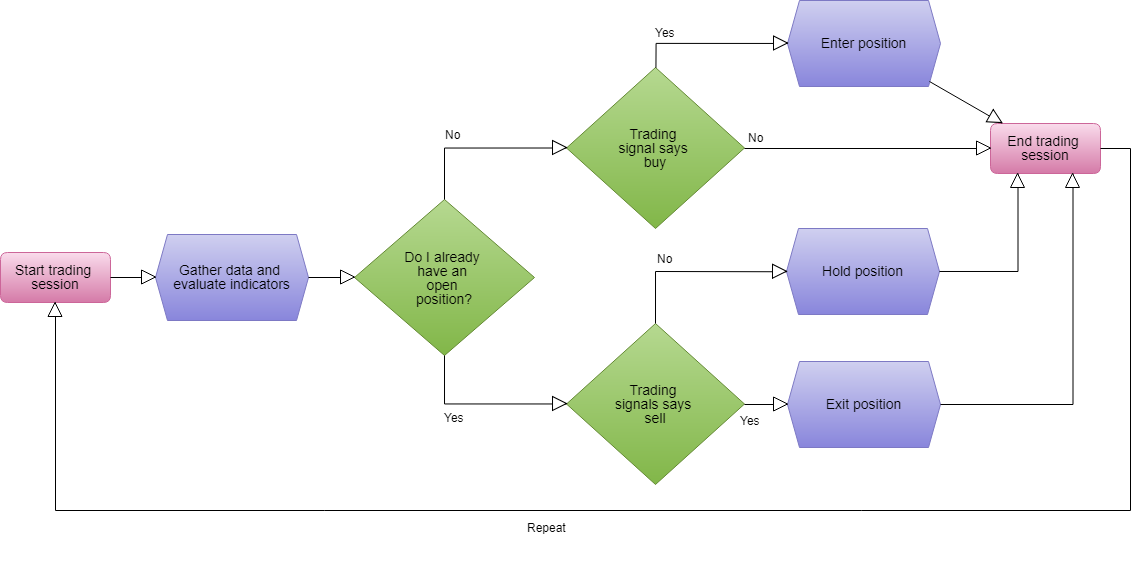
Simulation loop
The main piece of the puzzle for backtesting is the simulation loop. It walks over our input price data day by day, evaluates our rules and creates a series of trades.
If we wrote the code ourselves it would look something like this:
for (const bar of inputSeries) {
	if (inPosition) {
		// We currently have an open position,
		// do we need to exit the position?

		// Evaluate stop loss rule.
		evaluateStopLoss({ bar, position });

		// Evaluate exit rule.
		evaluateExitRule({ bar, position });
	}
	else {
		// We currently have no open position,
		// do we need to open a new position?

		// Evaluate entry rule.
		evaluateEntryRule({ bar });
	}
}
This code snippet is really just pseudo-code, Grademark actually provides the simulation loop for us. With Grademark we simply call the backtest function and pass in the input data and a JavaScript object that represents our trading strategy:
const { backtest } = require('grademark');

const trades = backtest(strategy, inputSeries);
The strategy object contains the functions entryRule, exitRule and stopLoss that define our strategy. The complete strategy definition looks like this:
const strategy = {
	entryRule: (enterPosition, args) => {
	   if (args.bar.close < args.bar.sma) {
		   enterPosition(); // Buy when price is below average.
	   }
	},

	exitRule: (exitPosition, args) => {
	   if (args.bar.close > args.bar.sma) {
		   exitPosition(); // Sell when price is above average.
	   }
	},

	stopLoss: args => {
	   // Stop out on 2% loss from entry price.
	   return args.entryPrice * (2 / 100);
	}
};
Capturing trades
The process of backtesting generates trades. The result of the backtest function captures the important data about each trade including entry and exit dates, entry and exit prices and the amount of profit per trade. Here’s an extract from Grademark’s TypeScript interface for a trade:
export interface ITrade {

	entryTime: Date;

	entryPrice: number;

	exitTime: Date;

	exitPrice: number;

	profit: number;

	profitPct: number;

	// ... More fields ...
}
Profit and other metrics are computed and attached to each trade object.
Analyzing the performance of the strategy
To understand the global performance of our strategy we might use Data-Forge and compute the sum of profit over all the trades:
const totalProfit = new DataFrame(trades)
   .deflate(trade => trade.profit)
   .sum();
However, Grademark provides an analyze function that does this and more:
const { analyze } = require('grademark');

const analysis = analyze(10000, trades);
The analyze function is passed an amount of starting capital and the set of trades. In this example, we are funding our virtual trading with a $10,000 account. The analysis loops over the trades and simulates trading with the requested amount of capital. Profitable trades increase the size of our account, losing trades decrease the size of our account. The result is a performance summary of our trading strategy that includes total profit and other useful metrics:
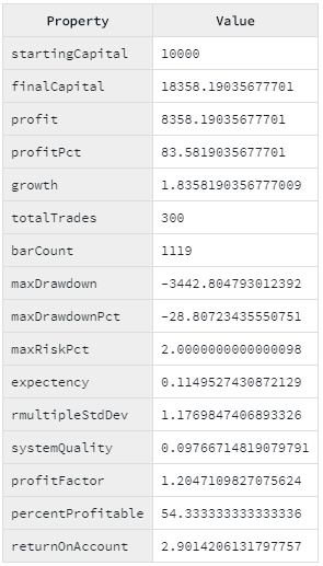
We now have a basic idea of how good (or bad) our strategy is. We can use this information to work out if the profit (83%) is worthwhile compared to the max risk (2%) or maximum drawdown (-28%).
We can now ask questions like can I tolerate a -28% drawdown? That’s jargon. Think of it this way: can I handle a 28% loss from the peak. As traders, a bit of forward planning like this really helps avoid situations where we might panic and pull out of a strategy before it manifests the anticipated profit.
We can use the analysis to determine if changes to a strategy will improve it or make it worse. The analysis also allows a comparison between alternate strategies that we might be considering.
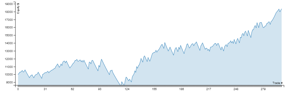
Visualizing equity and drawdown
After backtesting, it’s very common to render an equity curve for our strategy. The equity curve shows us the value of our trading account increasing over time:
Another useful chart shows the drawdown of our strategy over time. With the drawdown chart we can see the amount of time our strategy spends underwater:
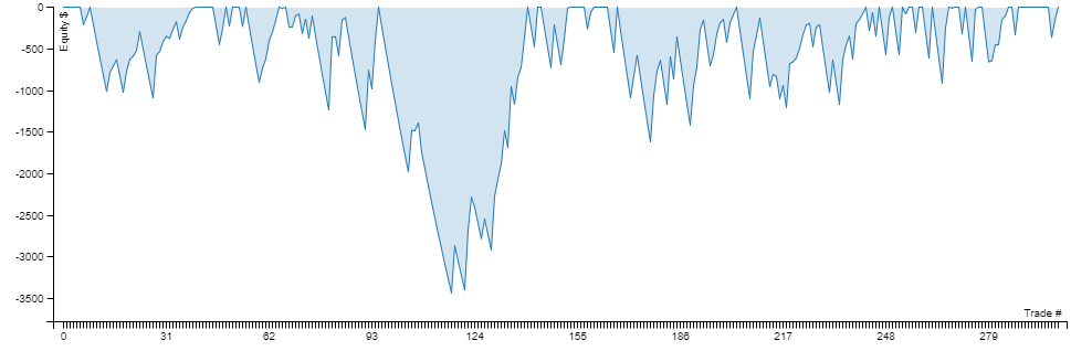
Such charts are produced by calling the Grademark functions computeEquityCurve and computeDrawdown and then plotting charts using tbe Plot library or Data-Forge Notebook:
const equityCurve = computeEquityCurve(10000, trades);
const equityCurvePlot = plot(
   equityCurve,
   {
       chartType: "area",
       y: { min: 9500, label: "Equity $" },
       x: { label: "Trade #" }
   }
);
await equityCurvePlot.renderImage("equity-curve.png");

const drawdown = computeDrawdown(10000, trades);
const drawdownPlot = plot(
   drawdown,
   {
       chartType: "area",
       y: { label: "Equity $" },
       x: { label: "Trade #" }
   }
);
await drawdownPlot.renderImage("drawdown.png");Conclusion
This post has been a basic overview of simulating and backtesting a simple example (mean reversion) trading strategy using JavaScript and the Grademark API.
This is just a starting point and we still have much more work to do. For instance, we haven’t taken into account the effect of fees or slippage. That means the results we are getting are probably too optimistic.
Also, our analysis is only based on one sequence of trades that would have occurred in the past and so far our use of data science has been simple and the results are quite fragile. We can’t expect to have this exact same performance again in the future because we’ll never again see this exact same sequence of trades. Fortunately, we have statistical tools we can throw at this problem like monte-carlo simulation. Monte-carlo simulation will help us have a better statistical understanding of what range of performance we can expect in the future from our trading strategy.
In addition, how do we know we are using the best parameters for our indicators? In this example trading strategy we used 30 days as a parameter to our moving average. Why 30 days? Why not some other number? Could a different value produce better (or worse) performance? We can use a process called walk-forward optimization, a kind of data-mining, to help us determine the performance impact of different parameter values for our trading strategy.
As you can see there are more advanced aspects of trading simulation and quantitative trading that I will write about in the future.
For more content like this, follow Ashley Davis on Twitter.
Support Ashley’s new book Backtesting and algorithmic trading with JavaScript.