
When it comes to using machine learning in the stock market, there are multiple approaches a trader can do to utilize ML models. From determining future risk to predicting stock prices, machine learning can be used for virtually any kind of financial modeling.
In our previous articles, we delved into the usage of two Time Series models: SARIMAX and Facebook Prophet. We utilized both of these models to forecast the potential, future prices of Bitcoin. Check out the following article if you are interested: https://towardsdatascience.com/predicting-prices-of-bitcoin-with-machine-learning-3e83bb4dd35f
In another article, we used classification models to classify stocks based on their performance in quarterly reports. You can read about the entire process of how we engineered different features from these reports and trained our classification models to determine investment decisions in the article below: https://medium.com/swlh/teaching-a-machine-to-trade-stocks-like-warren-buffett-part-i-445849b208c6
These are just a couple examples of how we can utilize machine learning models for financial markets.
In these articles, we just used models to predict future prices, however, that is just half the battle. The next step is how do we evaluate these models if they were to actually be used while trading? The answer to that question is called — Backtesting.
Backtesting
What is backtesting? Backtesting is the process of applying a trading strategy, predictive model, or analytical method to historical data to evaluate its accuracy and performance.
It is very important to note that backtesting does not 100% accurately, represent live-trading in the past. However, you should only use it to inform your decision to live-trade your strategy or not. Even then, it may be more practical to forward-test your strategy before trading with real money.
When we create a machine learning model, we need to backtest the model in order to determine how well it would have potentially performed in the past by feeding it historical data. There are two approaches when it comes to backtesting — Event-Driven and Vectorized Backtesting.
Vectorized Backtesting
Today, we will be using vectorized backtesting in order to evaluate the performance of our machine learning model. This approach allows us to quickly observe how our ML model might have performed in the past. If you would like to learn more about vectorized backtesting, then we suggest reading the following article by a machine learning researcher which contributed to the outcome of this current project: https://towardsdatascience.com/backtest-trading-strategies-with-pandas-vectorized-backtesting-26001b0ba3a5
Coding Our Machine Learning Model
In order to evaluate the performance of a machine learning model, we’ll first have to construct it in Python. The model we will be using is the AutoARIMA time series model from the pmdarima Python library. This model will quickly find the optimum parameters for us so we won’t need to worry about adjusting any modeling parameters.
However, if you do want to learn more about the parameters and what they mean, check out our previous article mentioned above that uses time series modeling to predict Bitcoin prices.
Step 1. Importing Necessary Libraries
import pandas as pd
import numpy as np
from pmdarima.arima import AutoARIMA
import plotly.express as px
import plotly.graph_objects as go
from tqdm.notebook import tqdm
from sklearn.metrics import mean_squared_error
from datetime import date, timedelta
import yfinance as yf
Each library here serves an important purpose for building and backtesting our ML model.
Step 2. Getting the Data
# Getting the date five years ago to download the current timeframe
years = (date.today() - timedelta(weeks=260)).strftime("%Y-%m-%d")

# Stocks to analyze
stocks = ['GE', 'GPRO', 'FIT', 'F']

# Getting the data for multiple stocks
df = yf.download(stocks, start=years).dropna()

# Storing the dataframes in a dictionary
stock_df = {}

for col in set(df.columns.get_level_values(0)):

    # Assigning the data for each stock in the dictionary
    stock_df[col] = df[col]
The data we will be using is a small collection of stocks with about 260 weeks of historical data. To be even less biased towards the performance of our model, we used stocks that have decreased in value in the past few years.
Another option for acquiring such data is through a financial data API such as EOD Historical Data, which has more than just historical price data. It is free to sign up and you’ll have access to vast amounts of financial data. Disclosure: I earn a small commission from any purchases made through the link above.
Step 3. Preprocessing the Data
# Finding the log returns
stock_df['LogReturns'] = stock_df['Adj Close'].apply(np.log).diff().dropna()
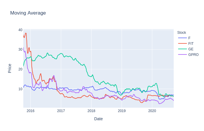
# Using Moving averages
stock_df['MovAvg'] = stock_df['Adj Close'].rolling(10).mean().dropna()
# Logarithmic scaling of the data and rounding the result
stock_df['Log'] = stock_df['MovAvg'].apply(np.log).apply(lambda x: round(x, 2))First, we’ll get the log returns for ours stocks, which we used later on to determine overall returns. Next, a 10-day moving average was applied to the dataset in order to smooth out and reduce the noise in closing prices. Finally, we scaled the moving averages by using a logarithmic scale rounded to 2 decimal places.
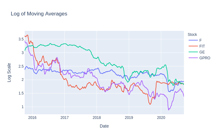
The reason we used moving averages and logarithmic scaling is because we hope that these values will be better suited for our model to predict prices much more accurately. There is no right answer in preprocessing or transforming the data to feed into our model so feel free to experiment with other scales, moving average windows, opening prices, etc.
Step 4. Training and Predicting with AutoARIMA
In order to run our model to get predictions with AutoARIMA, we will first layout all the requirements we want from our model and how to achieve them. Those things will be:
- Number of days to train with — Let’s use about a half year’s worth of data from the past closing prices.
- Number of days to predict — Let’s predict the next 5 days into the future for our forecast amount and then use the last day as the price target for our trading strategy.
- When and how often will the model run — Let’s run the model every other day or whenever the current price reaches or passes the price target.
- What date range we want to evaluate — We can set whatever range we like to backtest our ML model. Feel free to use whatever range you want but be aware that the bigger the range, the longer the training will take.
All of these values can be tinkered with. Feel free to try out different values to potentially find an amount that works best with this trading strategy.
After we run the code above, we will be given a DF of predictions for every stock in our portfolio. We will use these predictions for our backtest but let’s visualize them first.
Visualizing the Model’s Predictions
# Shift ahead by 1 to compare the actual values to the predictions
pred_df = stock_df['Predictions'].shift(1).astype(float).dropna()
Let’s create a new DataFrame for our predictions but with some alterations. We’ve shifted the predictions forward by one day so that our predictions will hopefully not suffer from look-ahead bias.
Here we iterate through each stock and visualize the predicted and actual values
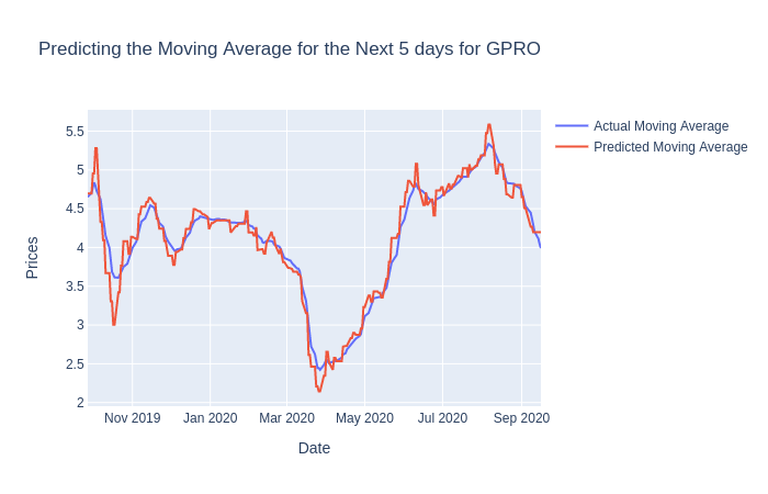
We can see that our model seems to do well enough but remember that the predictions are based on the last predicted day and serve as price targets in our trading strategy.
Evaluating the Predictions
Now that we’ve seen the differences between the actual values and the predicted values, we can quickly evaluate it’s quality by using the Root Mean Square Error to see how far off our predictions are.
for stock in stocks:

    # Finding the root mean squared error
    rmse = mean_squared_error(stock_df['MovAvg'][stock].loc[pred_df.index], pred_df
[stock], squared=False)

print(f"On average, the model is off by {rmse} for {stock}\n")
The Trading Strategy for the Model
Our strategy for our model is simple:
- Buy — When the predicted price target shows a significant increase from the current price.
- Sell — When the predicted price target shows a significant decrease from the current price.
- Hold (or Do Nothing)— If the price target shows neither a significant increase or decrease from the current price.
For example: If we set our model to predict 10 days in advance, then the last day’s predicted amount is the price target. If the price target is $103 and the current closing price is $100, then we will buy that stock because its price is predicted to increase by 3% in the next 10 days.
However, if the current price exceeds the predicted price target sooner than expected, then we can run the model again for a newer price target.
Let’s create a function that will establish positions in our backtest based on the strategy above:
def get_positions(difference, thres=3, short=True):
    """
    Compares the percentage difference between actual
    values and the respective predictions.

    Returns the decision or positions to long or short
    based on the difference.

    Optional: shorting in addition to buying
    """

    if difference > thres/100:

        return 1


    elif short and difference < -thres/100:

        return -1


    else:

        return 0
Positions Based on Model Predictions
Now using our function to establish positions, we can begin the backtesting portion of our model and trading strategy. We will need to create another DataFrame containing the Log Returns to use and the percentage difference between our predicted and actual values.
If you noticed in the “Positions” DF, we have shifted the series of positions by 2 days. This is done to account for look-ahead bias as well as the situation in which we may find ourselves deciding to initiate a trade closer to the end of the trading day based on the prediction from the day before. If we decided to initiate a trade at the very beginning of the trading day, then we may be fine with just shifting positions by 1 day instead.
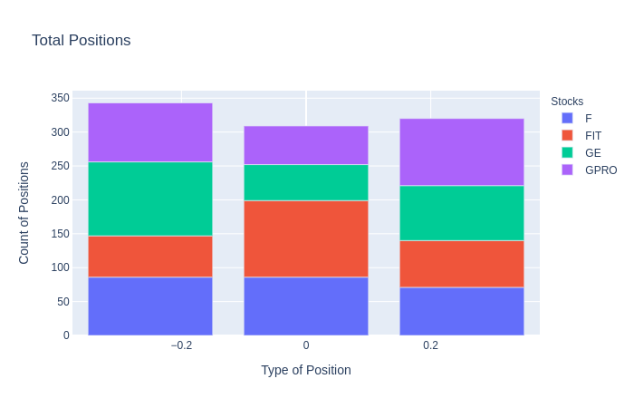
Plotting the Positions
Once we have established the positions in our backtest, we can then count the number of positions, the type of position, and which stock they belonged to. This is done to further analyze how often our strategy determines each position.
Vectorized Backtesting the Model
With our trading DataFrame ready to go, we can use vectorized backtesting and quickly visualize the returns for each individual stock and the returns from the overall portfolio.
Returns for Each Stock
# Calculating Returns by multiplying the
# positions by the log returns
returns = trade_df['Positions'] * trade_df['LogReturns']

# Calculating the performance as we take the cumulative
# sum of the returns and transform the values back to normal
performance = returns.cumsum().apply(np.exp)

# Plotting the performance per stock
px.line(performance,
        x=performance.index,
        y=performance.columns,
        title='Returns Per Stock Using ARIMA Forecast',
        labels={'variable':'Stocks',
                'value':'Returns'})
This code yields the following output for our vectorized backtest:
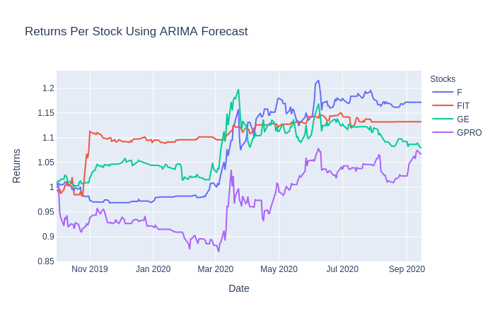
From this visualization, we can see that our ARIMA model strategy performs better with some stocks compared to others. With most of the stocks, you can see a significant jump right around March due to COVID’s effect on the market.
Returns on the Portfolio
In order to really evaluate our portfolio returns, we will need to compare our results with SPY. If we are capable of beating SPY returns, then our model shows promise and may be considered for forward-testing or live trading.
And here’s the result:
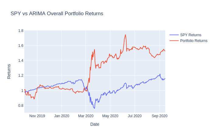
As you can see, our model initialy under-performs when compared to the SPY returns. However, it begins to beat SPY at the start of the stock market crash due to COVID. Feel free to change several values here and there within the model and within the strategy if you wish to achieve a different outcome.
Closing Thoughts
When we used this AutoARIMA model in combination with our simple stock trading strategy, we were able to achieve a better return performance than if we had just invested in SPY. However, we were able to perform pretty well at the end possibly due to the sudden stock market crash.
If we backtested on a different time frame or with different stocks, then it’s very probable we would not have achieved similar results. At this point, it’s a smart move to begin forward-testing this strategy in order to gain a better understanding of our model’s true performance.