

Combining two different forms of machine learning is a very exciting concept, especially when it comes to making money. In this case, I combined time series machine learning models with a sentiment analyzer. Two separate forms of machine learning used to create trade signals in the cryptocurrency market. This wasn’t the first time I’ve attempted to do this and it probably won’t be my last.
In my previous articles, I’ve used Facebook Prophet to forecast Bitcoin prices and sentiment analysis on Tweets to predict stock price movement. However, I have yet to fuse both of these methods together. But, even that statement is not entirely true. Recently, I combined Facebook Prophet with sentiment analysis on financial news headlines, but not tweets. So this time around, I will be experimenting with the slightly altered approach of using tweet sentiment.
Anyways — let’s dive right in and learn how I backtested a trading strategy using Facebook Prophet and Twitter sentiment analysis! Feel free to code along if you wish, I’ll also provide my code on Github for reference at the end of this article.
Importing Libraries
from eod import EodHistoricalData
import pandas as pd
from datetime import datetime, timedelta
from tqdm import tqdm
import twint
import nest_asyncio
nest_asyncio.apply()
from nltk.sentiment.vader import SentimentIntensityAnalyzer
import nltk
import numpy as np
import random
import plotly.express as px
from prophet import Prophet
I know it’s a lot of libraries, but it is what is needed in order for this backtest to run correctly. I will explain the two libraries above that you need in order to retrieve the data…
How to Get Crypto Price and Twitter Data
To get the price data, I used a financial data API from EOD-HD, which allows me to easily retrieve crypto price history from many different cryptocurrencies. It’s free to sign up and you’ll get your own API key in order to access the price history data. Disclosure: I earn a small commission from any purchases made through the link above.
# Importing and assigning the api key
with open("../../eodHistoricalData-API.txt", "r") as f:
    api_key = f.read()

# EOD Historical Data client
client = EodHistoricalData(api_key)
Next, I used Twint to easily retrieve the daily tweets regarding a specific crypto using their “cashtag”. No API key is needed for this one but I suggest reading up on their documentation in order to know how to properly access the data.
Retrieving Tweets and Price History
Now that I’ve established the required libraries to gather the data, I can code out the entire process of retrieving it. The first piece of data is a year’s worth of tweets regarding a specific cryptocurrency. In this case — Bitcoin.
Gathering Tweet on Bitcoin
Above, I created two functions. The first function (getTweets)configures Twint to retrieve tweets with specific parameters. For example, I wanted to filter out any unsubstantial tweets so I configured twint to query only popular tweets from verified users.
The second function (tweetByDay) implements getTweets in order to retrieve tweets on day by day basis. I used a recursive method for this function in order to retrieve the daily tweets from last year (2021). If you’re wondering why I decided to call the twint query multiple times instead of just once with a time frame of a year, it was because of my want of uniformity among tweets retrieved each day. In my experience with twint, there is a lack of consistency regarding tweets returned when it used on a longer time frame.
Anyways, here is how I called the twint query:
# Getting tweets daily
df = tweetByDay(
    start="2021-01-01",
    end="2022-01-01",
    df=pd.DataFrame(),
    search="$BTC",
    limit=20
)

# Saving file for later use
df.to_csv("tweets.csv")

# Reading file and saving to DF
tweet_df = pd.read_csv("tweets.csv", index_col=0)
Using twint in this case, may take awhile, so I opted to save the year’s worth of tweets as a CSV file for later use if needed.
Gathering Bitcoin Price History
Now that I have the year’s worth of tweets, I can now gather Bitcoin’s price history from around the same time frame:
With this function, I can gather the price history of Bitcoin that fits within the same time frame as the previously gathered Twitter data. In addition to gathering data from the same time frame, this function also gathers price history from further in the past in order to train FB Prophet as well as formatting the data to be compatible with Prophet.
Running Facebook Prophet
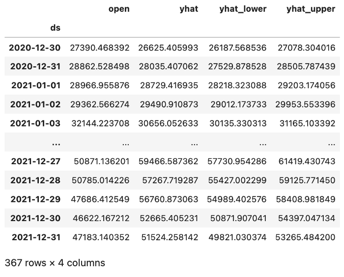
Now that I have the price history for Bitcoin, I can train Prophet to predict prices N days into the future. With the following functions I created, I’ll create a Pandas DataFrame containing the predictions containing the last day forecasted:
With the above functions, I can create the prediction DF using the following parameters:
# Pricing Data Parameters
training_days = 200

mov_avg = 3

forecast_period = 3

# Retrieving prices with the above parameters
prices = getPrices(
    "BTC",
    training_days=training_days,
    tweet_df=tweet_df,
    mov_avg=mov_avg,
    forecast_period=forecast_period
)
With these parameters (which can be changed to whatever you see fit) I created the DF of predictions below:
Running Tweet Sentiment Analysis
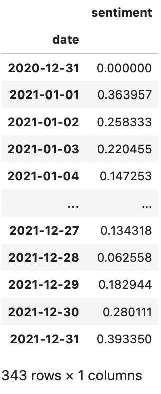
With the price predictions ready, I can move on to creating a DF consisting of the daily average sentiment score:
With the above function, I can analyze the sentiment of tweets for each day and return the average score for that day:
# Getting sentiment scores
sent_df = getSentiment(tweet_df)
Running this function returns a DataFrame of sentiment scores for the past year:
Getting Trade Positions
The next step is to establish trading positions for each DF. The following functions will form the trading positions for the price prediction DF, tweet sentiment DF, and the combination of both:
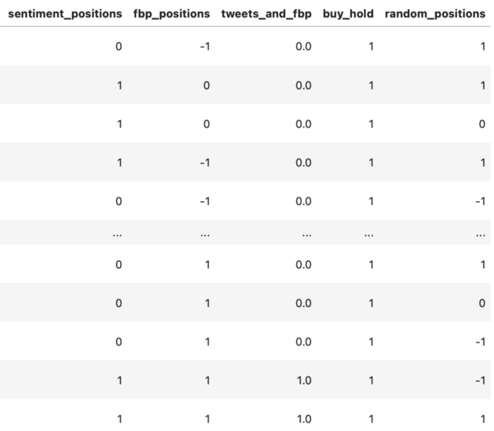
In the above functions, positions are set as 1, 0, -1 representing buy, hold/exit from previous position, and short. The sentimentPositions function has a customizable threshold parameter for the sentiment score which determines the given position. The fbpPosition function bases the positions on Prophet’s predicted upper and lower bound forecasts (yhat). The overallPositions function observes the positions set by the two previous functions and returns the same position if they both match. Below I applied all the functions to create a new positions DF:
# Applying the position function
sent_df['sentiment_positions'] = sent_df['sentiment'].apply(
    lambda x: sentimentPositions(x, thresh=0.2, short=True)
)

# Filling in missing days with the most recent position value
date_index = pd.date_range(sent_df.index[0], sent_df.index[-1])sent_df = sent_df.reindex(
    date_index,
    method='ffill'
)

# Converting index to string
sent_df.index = sent_df.index.map(lambda x: str(x)[:10])# Adding sentiment positions to the forecast DF
positions = pred_df.merge(
    sent_df,
    right_index=True,
    left_index=True,
    how='inner'
)

# Getting forecast prophet positions
positions['fbp_positions'] = positions.apply(
    lambda x: fbpPositions(x, short=True),
    axis=1
)

# Getting the overall positions of prophet and sentiment
positions['tweets_and_fbp'] = positions.apply(
    lambda x: overallPosition(x),
    axis=1
)

# Buy and hold position
positions['buy_hold'] = 1# Random positions
random.seed(123)
positions['random_positions'] = random.choices(
    [1,0,-1], k=len(positions)
)
Now each position for each day has been established in a new DF containing positions:
Backtesting each Strategy
Finally, I can perform the backtest using vectorized backtesting. To do so I need to get the log returns for the entire year of 2021 or at least the returns during the same time frame as the positions DF.
# Getting log returns during the time period set by the positions before
log_returns = prices[['ds', 'close']].set_index(
    'ds'
).loc[positions.index].apply(np.log).diff()
With the log returns, I can now perform the backtest by multiplying the log return values with the positions DF:
# The positions to backtest (shifted ahead by 1 to prevent lookahead bias)
bt_positions = positions[[
    'tweets_and_fbp',
    'buy_hold',
    'random_positions',
    'sentiment_positions',
    'fbp_positions'
]].shift(1)

# The returns during the backtest
returns = bt_positions.multiply(
    log_returns['close'],
    axis=0
)

# Inversing the log returns to get daily portfolio balance
performance = returns.cumsum().apply(
    np.exp
).dropna().fillna(
    method='ffill'
)
In order to compensate for any lookahead bias, I shifted the predictions ahead by 1 day. It is also why I used the “open” prices instead of “close” when determining trading positions. After the positions have been shifted, I multiplied the log returns with the DF containing the positions, calculated the cumulative sum of each strategy, then inversed the log returns.
The final performance of the backtest for each position is now stored within the performance variable, which will be visualized in the next section…
Backtest Visualization
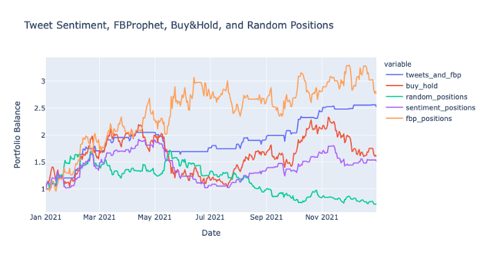
In the visualization above, you can see how well each strategy performed and the final portfolio balance at the end of the year. Let’s clear up the visualization by removing several of the other strategies in order to get a closer look at the Tweet & FBProphet strategy:
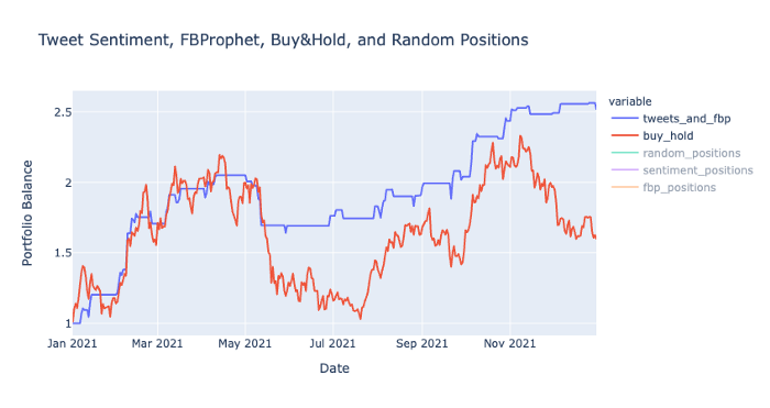
Here you can see the final performance of the combined strategy of tweet sentiment and Prophet compared to a regular buy and hold strategy.
Closing Thoughts
This tweet sentiment and Prophet strategy performed fairly well even compared to the simple buy and hold approach. Although it may have started out similar, the strategies later diverged with one eventually outperforming the other.
After running the backtest multiple times, I found this performance, based on the parameters I set above, to be one of the better performing backtests. Even though the Prophet positions strategy alone appeared to perform better, overall, it was still more volatile than the sentiment and Prophet strategy, albeit with a slightly higher ending balance. There could be other approaches or strategies to compare this performance to, however, these are probably the most obvious ones. If you feel like another strategy should be included, feel free to try it out yourself by referring to my code in my Github link below.
The next step, perhaps would be to take this strategy and forward test it with a small amount of capital but first I will need to build a trading bot integrated with a crypto exchange.