

I magine being able to know when a stock is heading up or going down in the next week and then with the remaining cash you have, you would put all of your money to invest or short that stock. After playing the stock market with the knowledge of whether or not the stock will increase or decrease in value, you might end up a millionaire!
Unfortunately, this is impossible because no one can know the future. However, we can make estimated guesses and informed forecasts based on the information we have in the present and the past regarding any stock. An estimated guess from past movements and patterns in stock price is called Technical Analysis. We can use Technical Analysis (TA)to predict a stock’s price direction, however, this is not 100% accurate. In fact, some traders criticize TA and have said that it is just as effective in predicting the future as Astrology. But there are other traders out there who swear by it and have established long successful trading careers.
In our case, the Neural Network we will be using will utilize TA to help it make informed predictions. The specific Neural Network we will implement is called a Recurrent Neural Network — LSTM. Previously we utilized an RNN to predict Bitcoin prices (see article below): https://towardsdatascience.com/predicting-bitcoin-prices-with-deep-learning-438bc3cf9a6f
In the article, we explored the usage of LSTM to predict Bitcoin prices. We delved a little bit into the background of an LSTM model and gave instructions on how to program one to predict BTC prices. However, we limited the input data to Bitcoin’s own price history and did not include other variables like technical indicators such as volume or moving averages.
Multivariable Input
Since the last RNN we constructed could only take in one sequence (past closing prices) to predict the future, we wanted to see if it would be possible to add even more data to the Neural Network. Maybe these other pieces of data could enhance our price forecasts? Perhaps by adding in TA indicators to our dataset, the Neural Network might be able to make much more accurate predictions? — Which is exactly what we want to accomplish here.
In the next few sections, we will be constructing a new Recurrent Neural Network with the capability to take in not just one piece but multiple pieces of information in the form of technical indicators in order to forecast future prices in the stock market.
Price History and Technical Indicators
In order to use a Neural Network to predict the stock market, we will be utilizing prices from the SPDR S&P 500 (SPY). This will give us a general overview of the stock market and by using an RNN we might be able to figure out which direction the market is heading.
Downloading Price History
To retrieve the right data for our Neural Network, you will need to head over to Yahoo Finance and download the prices for SPY. We will be downloading five years worth of price history for SPY as a convenient .csv file.
Another option would be to use a financial data API such as EOD Historical Data. It is free to sign up and you’ll have access to vast amounts of datasets. Disclosure: I earn a small commission from any purchases made through the link above.
Technical Indicators
After we have downloaded the price history for SPY, we can apply a Technical Analysis Python library to produce the Technical Indicator values. A more in depth look into the process from which we were able to retrieve the indicator values was covered here: https://towardsdatascience.com/technical-indicators-on-bitcoin-using-python-c392b4a33810
The article above goes over the exact TA Python library we utilized in order to retrieve the indicator values for SPY.
Coding the Neural Network
Import Libraries
Let’s begin coding out our Neural Network by first importing some libraries:
First, we imported some of the usual Python libraries (numpy, pandas, etc). Next, we imported the technical analysis library we previously utilized to create Technical Indicators for BTC (covered in the article above). Then, we imported the Neural Network library from Tensorflow Keras. After importing the necessary libraries, we’ll load in the SPY.csv file we downloaded from Yahoo Finance.
Preprocessing the Data
Datetime Conversion
After loading in the data, we’ll need to perform some preprocessing in order to prepare our data for the neural network and one of the first things we’ll need to do is convert the DataFrame’s index into the Datetime format. Then we will set the Date column in our data as the index for the DF.
Creating Technical Indicators
Next, we’ll create some technical indicators by using the ta library. To cover as much technical analysis as possible, we’ll use all the indicators available to us from the library. Then, drop everything else besides the indicators and the Closing prices from the dataset.
Recent Data
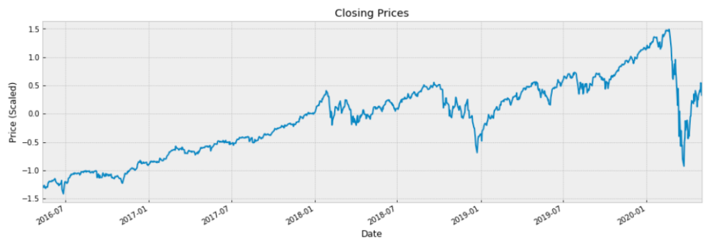
Once we have created the technical indicator values, we can then eliminate some rows from our original dataset. We will only be including the last 1000 rows of data in order to have a more accurate representation of the current market climate.
Scaling the Data
When scaling our data, there are multiple approaches to take to make sure our data is still accurately represented. It may be useful to experiment with different scalers to see their effect on model performance.
In our case, we will be utilizing RobustScaler to scale our data. This is done so that extreme outliers will have little effect and hopefully improve training time and overall model performance.
Helper Functions
Before we start constructing the neural network, let’s create some helper functions to better optimize the process. We’ll explain each function in detail.
split_sequence— This function splits a multivariate time sequence. In our case, the input values are going to be the Closing prices and indicators for a stock. This will split the values into our X and y variables. The X values will contain the past closing prices and technical indicators. The y values will contain our target values (future closing prices only).visualize_training_results— This function will help us evaluate the Neural Network we just created. The thing we are looking for when evaluating our NN is convergence. The validation values and regular values for Loss and Accuracy must start to align as training progresses. If they do not converge, then that may be a sign of overfitting/underfitting. We must go back and modify the construction of the NN, which means to alter the number of layers/nodes, change the optimizer function, etc.layer_maker— This function constructs the body of our NN. Here we can customize the number of layers and nodes. It also has a regularization option of adding Dropout layers if necessary to prevent overfitting/underfitting.validater— This function creates a DF with predicted values for a specific range of dates. This range rolls forward with each loop. The intervals for the range are customizable. We use this DF to evaluate the model’s predictions by comparing them to the actual values later on.val_rmse— This function will return the root mean squared error (RMSE) of our model’s predictions compared to the actual values. The value returned represents how far off our model’s predictions are on average. The general goal is to reduce the RMSE of our model’s predictions.
Splitting the Data
In order to appropriately format our data, we will need to split the data into two sequences. The length of these sequences can be modified but we will be using the values from the last 90 days to predict prices for the next 30 days. The split_sequence function will then format our data into the appropriate X and y variables where X contains the closing prices and indicators for the past 90 days and y contains the closing prices for the next 30 days.
# How many periods looking back to learn
n_per_in  = 90

# How many periods to predict
n_per_out = 30

# Features
n_features = df.shape[1]

# Splitting the data into appropriate sequences
X, y = split_sequence(df.to_numpy(), n_per_in, n_per_out)
What our NN will do with this information is learn how the last 90 days of closing prices and technical indicator values affect the next 30 days of closing prices.
Neural Network Modeling
Now we can begin constructing our Neural Network! The following code is how we construct our NN with custom layers and nodes.
This is where we begin experimenting with the parameters for:
- Number of Layers
- Number of Nodes
- Different Activation functions
- Different Optimizers
- Number of Epochs and Batch Sizes
The values we input for each of these parameters will have to be explored as each value can have a significant effect on the overall model’s quality. There are probably methods out there to find the optimum values for each parameter. For our case we subjectively tested out different values for each parameter and the best ones we found can be seen in the code snippet above.
If you wish to know more about the reasoning and concepts behind these variables, then it is suggested that you read our previous article about Deep Learning and Bitcoin.
Visualizing Loss and Accuracy
After training, we will visualize the progress of our Neural Network with our custom helper function:
visualize_training_results(res)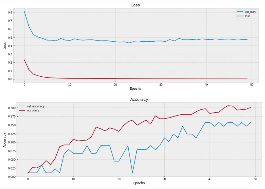
As our network trains, we can see that the Loss decreasing and Accuracy increasing. As a general rule, we are looking for the two lines to converge or align together as the number of epochs increases. If they do not, then that is a sign that the model is inadequate and we will need to go back and change some parameters.
Model Validation
Another way we can evaluate the quality of our model’s predictions is to test it against the actual values and calculate the RMSE with our custom helper function: val_rmse.
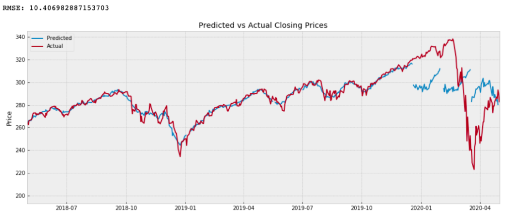
Here we plot the predicted values with the actual values to see how well the compare. If the plot of the predicted values are extremely off and nowhere near the actual values, then we know that our model is deficient. However, if the values appear visually close and the RMSE is very low, then we can conclude that our model is acceptable.
Our model seems to do well in the beginning but it cannot capture or model some intense movements in the price. This is probably why the last three predictions appear very far off. Perhaps with more training and experimentation our model could anticipate those movements.
Forecasting the Future
Once we are satisfied with how well our model performs, then we can use it to predict future values. This part is fairly simply relative to what we have already done.
Here we are just predicting off of the most recent values we have from the downloaded .csv file. Once we run the code we are presented with the following forecast:
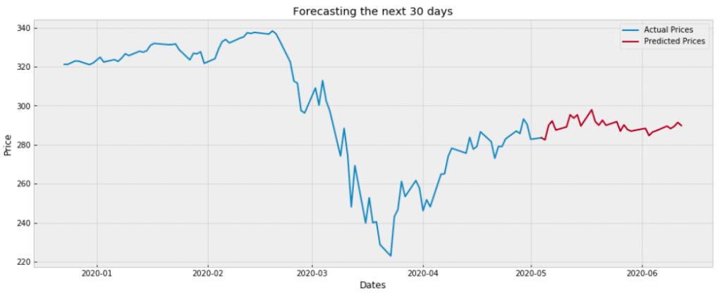
And there we have it! — The forecasted prices for SPY. Do what you wish with this knowledge but remember one thing: the stock market is unpredictable. The values predicted here are not certain. They may be better than just randomly guessing since the values are educated guesses based on the Technical Indicators and price patterns from the past.
Closing
We were able to successfully construct a Recurrent Neural Network of LSTM layers that is able to take in multiple inputs rather than just one. The quality of the model may vary from person to person depending on how much time they wish to spend on it. These predictions can be extremely useful for those wishing to gain some insight into the future price movement of a stock even though predicting the future isn’t possible. But, it is likely to believe that this way is better than randomly guessing.