

Fibonacci extensions and retracements in Python using financial trading data from EOD Historical Data (EODHD APIs) data API
The Fibonacci sequence is fascinating and a very popular topic for writers, mathematicians, and the lik
If you want to learn how to install the EODHD APIs Python Financial Official Library and activate your API key, we recommend to start with exploring of our Documentation for it.
At a high level, it is a series of numbers in which each number (the Fibonacci numbers) are the sum of the two preceding numbers. The series starts with 1, 1, 2, 3, 5, 8, 13, 21, etc.
As the numbers get larger, the quotient between each successive pair of Fibonacci numbers is very close to 1.618, or its inverse 0.618. This is most commonly referred to as the Golden Ratio.
The Golden Ratio very interestingly appears in some patterns in nature, including spiral arrangements of leaves, number of flower petals, the structure of tree branches, and other plant life. It is also used to analyse artificial systems such as financial markets, which is the main focus on this article.
Golden ratio in Fibonacci sequence: 8/13 = 0.618 (61.8%), 21/34 = 0.618 (61.8%), 34/55 = 0.618 (61.8%), 55/89 = 0.618 (61.8%), etc.
Mathematicians started investigating other ratios which may be connected to the Fibonacci sequence.
Fibonacci Retracement and Extensions for Trading in Python
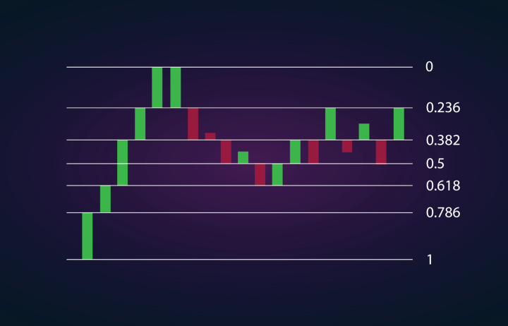
Fibonacci retracement measures the percentage of how much of a correction may happen after a price movement.
The Fibonacci retracement levels are 23.6%, 38.2%, 50%, 61.8%, 78.6%, 100% with extension levels at 138.2%, 161.8%, 200%, and 261.8%.
If we take the Fibonacci sequence 0, 1, 1, 2, 3, 5, 8, 13, 21, 34, 55, 89; and divide 55/89 we get 0.618, divide 34/89 we get 0.382, divide 21/89 we get 0.236, etc. The square root of 0.618 is 0.786. While not officially a Fibonacci ratio, 50% is also used.
This indicator is useful because it can be drawn between any two significant price points, such as a high and a low in trading. On trading graphs they look like support and resistance levels.
Fibonacci extensions use similar percentages but for a different purpose. They are a way to predict a target price to sell or find potential areas of support or resistance when the price is moving into unchartered territory.
Calculating Fibonacci levels in Python for trading
We’re going to need to retrieve some trading data. I’ll be using my trusty financial data API provider EODHD APIs, previously EOD Historical Data. I have a paid for account as I use it often but there is a free tier if you want to use that instead and follow along.
I’ll be using Google Colab notebooks to demonstrate this. It’s free and easy to use. It will allow you to run Python code snippets without having to install anything locally.
I use Python a lot for trading data analysis. I wrote an article previously to help those get set up. It has instructions on how to use Google Colab, which we will be using here. If you want to do this locally on your desktop, it will work fine as well.
Let’s start by retrieving some data to work with…
I’m going to use the S&P 500 (GSPC.INDC or ^GSPC) interday index using the EODHD API’s Python library in Google Colab. This index is amazing to trade but data providers never offer it for free. If you want to access this data you will need a subscription. If you want to try it out for free they have a demo API key which allows you to access Apple’s stock data using the AAPL stock code.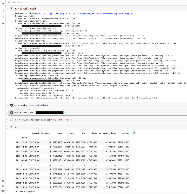
We now have 207 days of S&P 500 data stored in a Pandas dataframe called “df”. We can now graph it like this.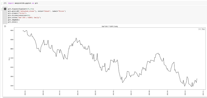
In order to perform our Fibonacci retracement calculations, we’re going to need the following:
- The highest price in the focus range
- The lowest price in the focus range
- If the market is in an uptrend or downtrend
To get the high and low is easy…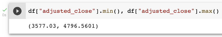
The S&P 500 currently visually looks like it’s in a downtrend. If you want to be sure you can do something like this.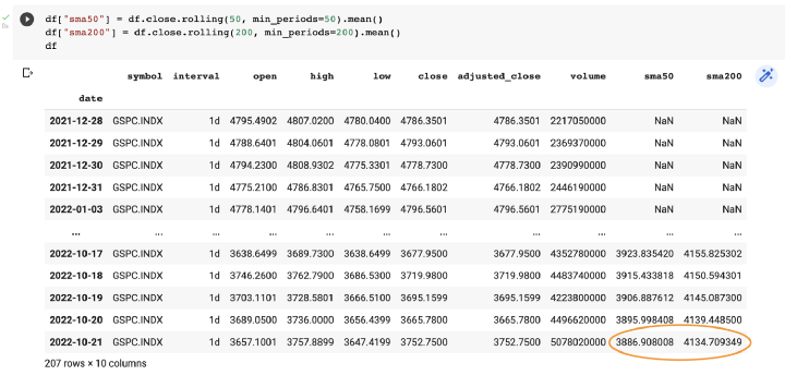
I’ve added two simple moving averages to our dataset, SMA50 and SMA200. The SMA50 is the 50-day rolling average and the SMA200 is the 200-day rolling average. The SMA50 is currently below the SMA200 on the 21st of October 2022, which is indicating a long term downtrend.
The question we are trying to answer now is how far this downtrend will go and potential places it may improve. This is where Fibonacci retracement levels can be really useful for Trading in Python.
The calculations are as follows:
Uptrend Retracement = High - ((High - Low) * Percentage)

Uptrend Extension = High + ((High - Low) * Percentage)

Downtrend Retracement = Low + ((High - Low) * Percentage)

Downtrend Extension = Low -((High - Low) * Percentage)
We will be using the “Downtrend Retracement” formula.
Low + ((High - Low) * Percentage)
23.6% = 3577.03 + ((4796.5601 - 3577.03) * 0.236)
23.6% = 3577.03 + (1219.5301 * 0.236)
23.6% = 3577.03 + (1219.5301 * 0.236)
23.6% = 3577.03 + 287.8091036
23.6% = 3864.8391036
We then repeat this process with the other Fibonacci percentages. To do this programmatically we can do this.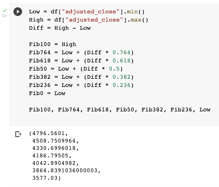
For your convenience, here is the Google Colab code.
Low = df["adjusted_close"].min()
High = df["adjusted_close"].max()

Diff = High - LowFib100 = High
Fib764 = Low + (Diff * 0.764)
Fib618 = Low + (Diff * 0.618)
Fib50 = Low + (Diff * 0.5)
Fib382 = Low + (Diff * 0.382)
Fib236 = Low + (Diff * 0.236)

Fib0 = LowFib100, Fib764, Fib618, Fib50, Fib382, Fib236, Low
And this is how we plot it in Matplotlib.
plt.figure(figsize=(30,10))
plt.plot(df["adjusted_close"], color="black", label="Price")
plt.axhline(y=Fib100, color="limegreen", linestyle="-", label="100%")
plt.axhline(y=Fib764, color="slateblue", linestyle="-", label="76.4%")
plt.axhline(y=Fib618, color="mediumvioletred", linestyle="-", label="61.8%")
plt.axhline(y=Fib50, color="gold", linestyle="-", label="50%")
plt.axhline(y=Fib236, color="darkturquoise", linestyle="-", label="23.6%")
plt.axhline(y=Fib0, color="lightcoral", linestyle="-", label="0%")

plt.ylabel("Price")
plt.xticks(rotation=90)
plt.title("S&P 500 (^GSPC) Daily")
plt.legend()
plt.show()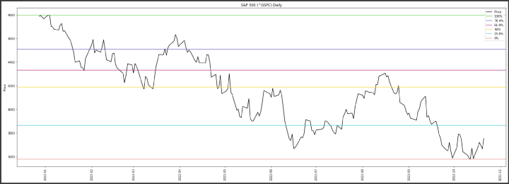
Fibonacci extensions would be calculated like this (for an uptrend).
Fib2618 = High + (Diff * 2.618)
Fib2000 = High + (Diff * 2)
Fib1618 = High + (Diff * 1.618)
Fib1382 = High + (Diff * 1.382)
Fib1000 = High + (Diff * 1)
Fib618 = High + (Diff * 0.618)
The Pandas dataframe is showing 207 days of data, but maybe we are only interested in data from mid-August. The Fibonacci retracement calculation only needs a high and low value. We can truncate our data as follows.
df_subset = df.tail(48)

plt.figure(figsize=(30,10))
plt.plot(df_subset["adjusted_close"], color="black", label="Price")
plt.ylabel("Price")
plt.xticks(rotation=90)
plt.title("S&P 500 (^GSPC) Daily")
plt.legend()
plt.show()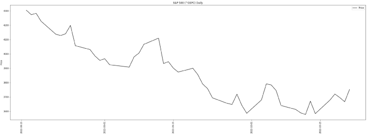
We will calculate our new levels like this.
Low = df_subset["adjusted_close"].min()
High = df_subset["adjusted_close"].max()
Diff = High - Low

Fib100 = High
Fib764 = Low + (Diff * 0.764)
Fib618 = Low + (Diff * 0.618)
Fib50 = Low + (Diff * 0.5)
Fib382 = Low + (Diff * 0.382)
Fib236 = Low + (Diff * 0.236)
Fib0 = Low

Fib100, Fib764, Fib618, Fib50, Fib382, Fib236, Low
And plot our new data.
plt.figure(figsize=(30,10))
plt.plot(df_subset["adjusted_close"], color="black", label="Price")
plt.axhline(y=Fib100, color="limegreen", linestyle="-", label="100%")
plt.axhline(y=Fib764, color="slateblue", linestyle="-", label="76.4%")
plt.axhline(y=Fib618, color="mediumvioletred", linestyle="-", label="61.8%")
plt.axhline(y=Fib50, color="gold", linestyle="-", label="50%")
plt.axhline(y=Fib236, color="darkturquoise", linestyle="-", label="23.6%")
plt.axhline(y=Fib0, color="lightcoral", linestyle="-", label="0%")

plt.ylabel("Price")
plt.xticks(rotation=90)
plt.title("S&P 500 (^GSPC) Daily")
plt.legend()
plt.show()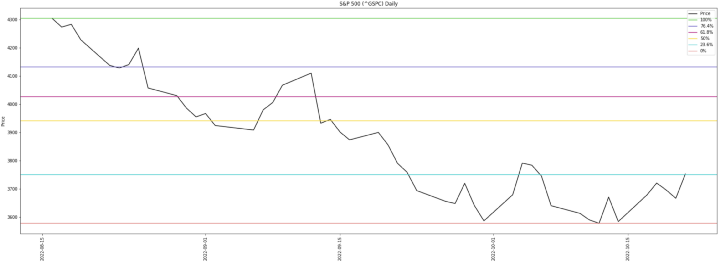
As you can see the Fibonacci retracement levels form a sort of support and resistance.
EODHD API’s Python Library
I pushed an update to the EODHD API’s Python library to make this functionality easily available to everyone. It’s available from version 1.0.8.
Retrieve our data as before, or any data you like.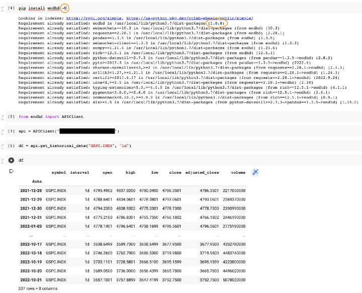
Two important points to mention here:
- I used the -U argument for my PIP install to make sure that my current “eodhd” library upgrades to the latest version
- I confirmed the version I’m using on Google Colab is 1.0.8
So now the new exciting part!
from eodhd import EODHDGraphs
graphs = EODHDGraphs()
We can how render all our graphs as follows….
graphs.fibonacci_retracement(df, "downtrend", "adjusted_close")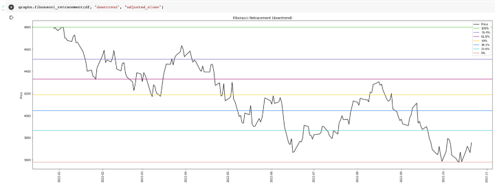
graphs.fibonacci_retracement(df, "uptrend", "adjusted_close")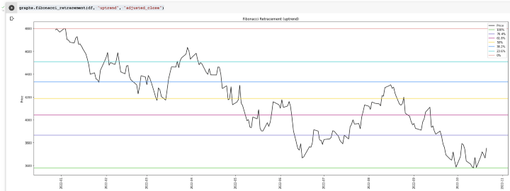
graphs.fibonacci_extension(df, "uptrend", "adjusted_close")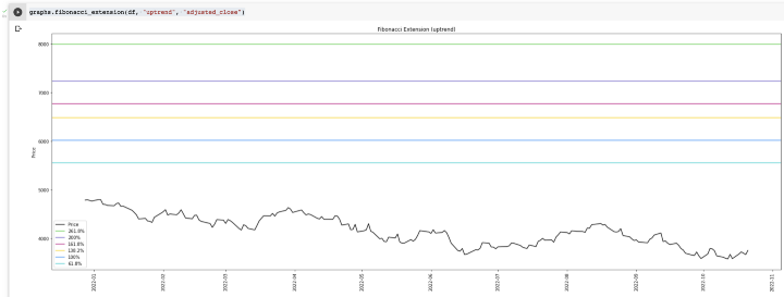
graphs.fibonacci_extension(df, "downtrend", "adjusted_close")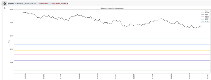
By default, the graphs will display without saving the graph. I’ve added two optional arguments to both functions.
- save_file=”fibonacci.png” ← default is “” which doesn’t save a file
- quiet=True ← default is False which displays the graph
This is how you can save the graph without displaying it.
I hope you enjoyed this article. If you did, please consider following me for future articles and clapping for the article as that helps remunerates me for my efforts 🙂